 Chances are that you won’t be using all of the data available in the DIY College Rankings spreadsheets. Once you’ve defined some basic filters, it’s generally a good idea to copy the data you want to work with to a different spreadsheet tab in the Excel workbook. This way you can add to or modify the data without accidentally deleting or creating errors in the original data. In this lesson, I’m going to show you the basics of how to copy data in Excel.
Insert a New Worksheet Tab
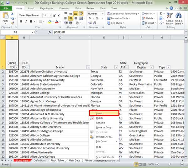
First, I’m going to enter a new worksheet to work with the data. Click on the tab you want to insert the new tab to the left of. In the following example, I click on Filters. Right click to bring up the menu.
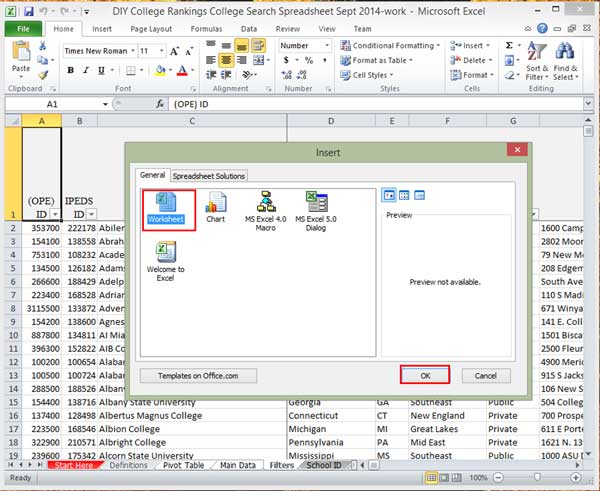
Select Insert and the Insert Dialog box will appear. Select Worksheet and then click the OK button.
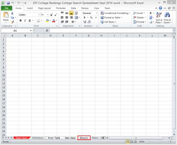
Excel creates a new worksheet called Sheet 1 to the left of the Filters tab.
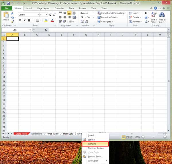
I’m going to give the worksheet a more meaningful name and rename it Work. Select the Sheet 1 tab, right click, and select Rename.
The text will be reversed highlighted. If you start typing, it will simply replace Sheet 1 with whatever you type. If you click while the text is highlighted what you type will be inserted rather than replaced. This means that you will have to use the delete key to get rid of the text you don’t want.
Copying Data
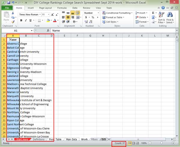
For the example, I’m going to show you how to copy data in Excel using just Wisconsin data. Go to the Filters tab and select just Wisconsin schools (see last lesson.)
Once the schools are selected, click on the column heading for the school names, in this case column C.
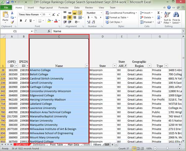
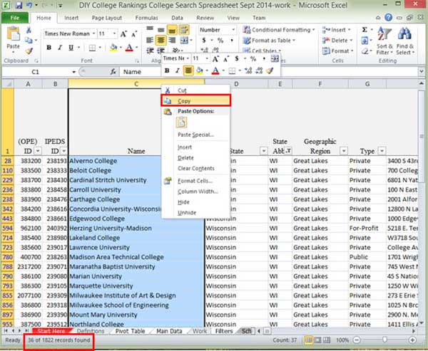
This selects the entire column, not just the cells with the data. If you scroll down, you’ll see that the entire column is selected. Next, right click to copy column c, the Name column.
You can see how many records you are copying in the bottom left-hand corner.
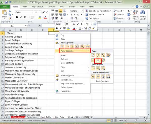
Excel will show the copied material outlined in dotted/moving lines. If you look in the bottom left hand corner, you’ll see instructions Select destination and press ENTER or choose Paste.
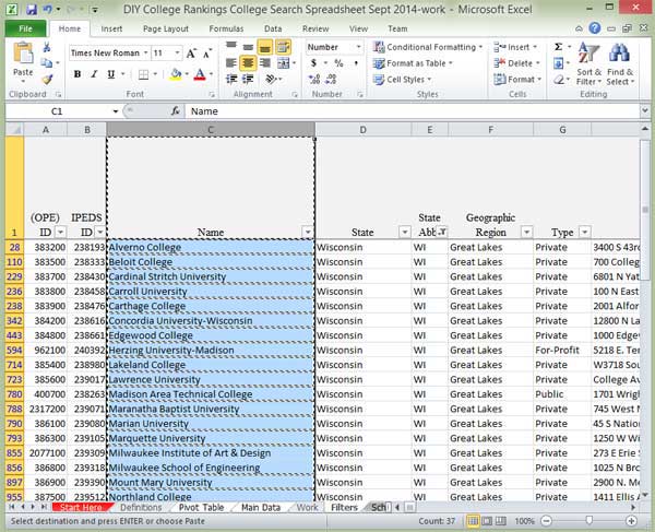
Next, click on the Work tab and press Enter.
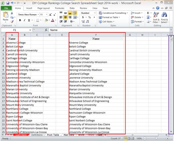
Notice that the column isn’t the same width. The names extend beyond the column boundaries. Excel gives you a lot of control over what you actually copy. When you copy data in Excel, the default is to copy everything, including the formatting and formulas, but not the column width.
Repeat the process of copying the column and click on the Work tab. Select the 1st cell of the F column. Right click to bring up your menu options. Then select Paste Special… and then Keep Source Column Widths icon.
This time you see that column width is copied as well.
How You Select Data For Copying
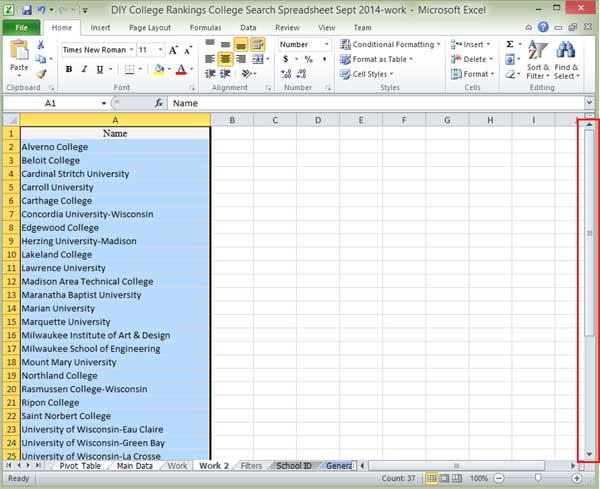
If you look at the vertical slider bar on the Work tab (purple in the above example), you’ll see a lot of space to scroll, much more than what is needed to scroll through the 37 records. This can actually be annoying depending on what you’re doing with the data.
This occurs because you copied the entire column, including all of the blank rows, not just the 37 rows you needed. In the following example, I’ll demonstrate how to copy data in Excel by selecting just the data needed.
Create a second worksheet and rename it to Work 2.
Select the top cell of the column you want to copy. In the example, I select the Name cell. Press the F8 key. You’ll see the status Extend Selection show up in the bottom left-hand corner. While the Name column is still selected, press the Control and Down Arrow keys at the same time.
![]()
Instead of selecting the entire column, Excel only selects to the end of the data in column. Copy the data as you did earlier and select the Work 2 tab. Right click and select Paste Special… with column widths.
Look at the vertical scroll bar. You’ll see that there is a lot less space to scroll through than in the original work tab.
Next week I’ll show you how to copy multiple columns. To get rid of the work tabs you created, select a tab, right-click and select Delete. Excel will warn you may be deleting data.
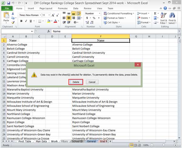
In this case, this is what we want to do so go ahead and select Delete.
5 thoughts on “Creating College Lists 101: Copying Data-Part 1”